Limited Population Growth

Part 2: Stepping Out: Rise = Rate x Run

Here is our procedure for generating a solution function P = P(t) for the initial value problem

• dP/dt = c P (M - P), and
• P = P₀ at time t = 0.

Starting from the known value P₀, we will generate a set of values

P₀ , P₁ , P₂ , P₃ , ..., P_n

at corresponding times

0 , t₁ , t₂ , t₃ , ..., t_n ,

where the times are equally spaced at (small) steps of Delta-t. In brief, we will use the fact that we know both P and dP/dt at time 0 to calculate a rise from P₀ to P₁. Once we have a value for P₁, we can find a slope at that point as well, so we can repeat the procedure to find P₂. Continuing in the same way, we can find as many values of P as we like. As we will see, the success of this procedure depends on how small our step sizes are, and, in any case, this is an approximation procedure, because we are using instantaneous rates of change as if they stay unchanged over each interval of length Delta-t.

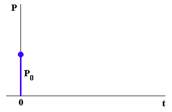
We illustrate the procedure graphically. The following diagram shows a graph of the starting situation. Plotting population as the dependent variable and time as the independent variable, the initial population P(0) is represented by a vertical line segment of length P(0) at the starting time t = 0.

Now we step forward in time to t₁ = Delta-t. We use the slope at time 0, which we call slope₀, to draw a line from (0, P₀) to (t₁, P₁):

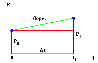
The slope of a line segment is the rise divided by the run, so the rise is the slope times the run. In our situation, the run is Delta-t, so

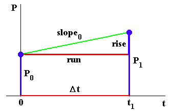
The line segment representing P₁ is the sum of two pieces, one of length P₀, and the other of length rise = slope₀ x Delta-t. Hence

Now enter the following formulas in your worksheet.

• The formula to compute P₁ from P₀.
• The same reasoning applies to computing P₂ from P₁. Enter the formula for P₂.
• The same reasoning applies to computing P_k from P_k-1. (See the next figure.) Enter the formula for P_k.

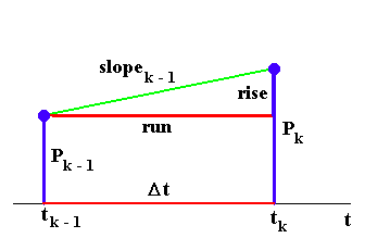
Great! It looks like we have a wonderful recursion relation for computing P_k from P_k-1, except for one little problem: What is slope₀? More generally, what is slope_k-1 for k = 1, 2, ... ? Answer: This is where our Theoretical Assumption from the Part 1 enters the picture! The assumption gives us a formula for the rate of change of population (the slope!) in terms of the current population.

• Use this observation to enter the formula for slope₀ in terms of P₀.
• The same reasoning applies to computing each slope_k from the corresponding P_k. Enter the resulting equation.

We thus have an interesting interweaving -- we have to compute our quantities in the following order:

P₀ , slope₀, P₁, slope₁, P₂, slope₂, P₃, slope₃, ..., P_n, slope_n.

We will put our formulas to use in the next Part.

Last modified: September 20, 1997