|
|
|
|
|
|
Part 4: Populations as Functions of Time
We saw in Part 3 that Euler's Method "works" for systems of differential equations the same way it does for a single equation -- but it doesn't work very well for tracking curves that have to loop around and come back where they started. The "default" differential equation solver in your helper application uses a more sophisticated technique than Euler's Method, but it's basically the same idea: Taking small steps in the time domain, predict as accurately as possible where the next x(t) and y(t) should be. The details of how to do that we leave to a module in the Differential Equations collection. But since we know the solver is there, we will use it for the rest of this module.
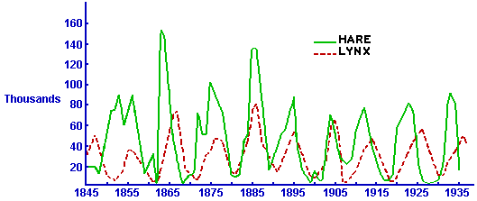
The same solver that generates pairs (x(t),y(t)) in the xy-plane can generate pairs (t,x(t)) in the tx-plane and (t,y(t)) in the ty-plane -- that is, solutions for the prey and predator populations as functions of time. Since we know the (x,y) pairs eventually repeat themselves, we must find x(T) = x(0) and y(T) = y(0) at some time t = T -- and then the coordinate functions start over through the same values. That is, x(t) and y(t) are both periodic functions with the same period T. On the other hand, the trajectories don't look much like circles or ellipses, so it will not be surprising if the population functions x(t) and y(t) don't look much like sines and cosines.

|
|
|
Last modified: November 11, 1997