Fourier Transform I

Part 3: Application to a Heat Problem

In this part, we will apply the Fourier transform to understand time evolution of temperature in an infinite rod. For simplicity, we are assuming that the thermal diffusivity constant a is 1. In this problem there is no boundary, thus no boundary conditions -- just the one-dimensional heat equation and an initial temperature distribution f.

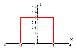
We assume that f is absolutely integrable. In fact, our first initial temperature distribution is graphed below

Suppose u(x,t) is the solution of this problem. Let U(w,t) be the Fourier transform of u with respect to x, i.e., for each t, we take the Fourier transform of the function of x obtained by holding t fixed and letting x vary. In particular, we have

where F is the Fourier transform of the initial temperature distribution function f.

We want to take the Fourier transform of the heat equation to obtain a corresponding condition on U. For t greater than 0, u(x,t) is continuous in x, so we know that the transform of a derivative may be obtained by multiplying the transform of the original function by iw. Thus, the Fourier transform of the second partial of u with respect to x is

Also, since we are taking the Fourier transform with respect to x, the transform of the partial of u with respect to t, may be shown to be just the partial of U with respect to t. So, after we transform, the problem becomes

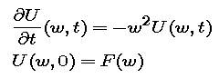
For each fixed w, this is just a simple first-order initial value problem in t.

Explain why the solution of this initial value problem is

In particular, explain where the factor F(w) comes from.

Now our problem is to find the inverse Fourier transform of U(w,t). We know that the Fourier transform of a convolution f * g is F(w) G(w), where F and G are the Fourier transforms of f and g respectively. In order to apply this to the particular inverse transform problem in front of us, we need to find a function g(x) such that its Fourier Transform is exp(-w²t). For this calculation we assume that t is fixed and positive.

Use your computer algebra system to find the Fourier transform of exp(- a x²), where a is assumed to be positive.
Determine values of a and b such that the Fourier transform of b exp(-a x²) is exp(-w²t). (Your values of a and b will depend on t.) Define g by
g(x) = b exp(-a x²)
where a and b have the values just determined.
Calculate and graph the convolution f * g for values of t between 0.01 and 30.
Examine the temperature/time surface -- the graph of u(x,t). Visually identify the curves graphed in Step 4 on this surface.
Describe in words the evolution of the temperature in the infinite rod as t increases from 0.01 to 30.

modules at math.duke.edu