The One-Dimensional
Heat Equation
Part 1: Equal Boundary
Conditions
We'll begin by experimenting
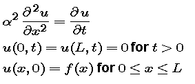
with an initial/boundary value problem of the form

Our starting values are alpha
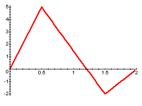
= 1 and L = 2. Here is a graph of the initial temperature distribution:

- Calculate the first 15
coefficients for the Fourier sine expansion for f. Then plot
the original function together with each of the first 15 Fourier approximations.
- How good are the approximations?
How do they change as the order of the approximation increases?
Now we look at the evolution
of the solution over time.
- Define the solution function
u(x,t) as a function of x with t as a parameter. Explain
how the particular values L = 2 and alpha = 1 determine the
symbolic form for the approximation.
- Vary t from 0.001
to 2.0 to see snapshots in time of the temperature distribution.
Take small time steps at first and then larger ones. Explain why the solution decays to the constant value 0. This explanation should be in terms of the symbolic form of the approximation -- not in terms of the underlying physical phenomenon.
- Explain why the temperature function reduces to a single arch as t increases -- again in terms of the symbolic form of the approximation.
modules at math.duke.edu

