Growth Models, Part 5.2

Population Growth Models

Part 5.2: Proportional Harvesting

For fishery management -- and many other harvesting situations -- it is unreasonable to assume that the harvest rate is constant (i.e., independent of the population). Generally speaking, the more fish, crabs, or lobsters in a given area, the more that will be caught. Thus, for modeling the Maine lobster fishery, we will assume that the harvest rate H is proportional to the population P.

We find it convenient to write the proportionality constant as the product of two components: a catchability quotient, which we denote by Q, and a measure of harvesting effort, which we call E. Q is a biological characteristic of the population -- not subject to human control -- but E is under the control of the lobstermen. Thus, our proportionality constant is Q times E, and our assumption about H is

H = Q E P.

Our new differential equation is then

where r, K, Q, and E are constants. This equation is not really new, because it can be written in the form

which is a logistic growth equation with a somewhat reduced value for the maximum supportable population.

Explain why the differential equation can be rewritten in the form just stated. Then explain why this equation is of the logistic form

In particular, what is M (in terms of K, Q, E and r), and how do we know that it is smaller than K?

This logistic model has only one nonzero equilibrium population, namely, M, and it will play a key role in our analysis. We are particularly interested in how M is related to the harvesters' effort E and to the corresponding harvest rate H.

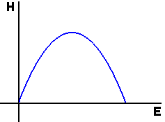
We first explore the effect that effort E has on the catch rate H. The relationship is not obvious, because E also influences the population P. To understand this relationship, we will assume that P has reached equilibrium. This is unlikely to be true -- since E is likely to change every year -- but it is a reasonable approximation, since solutions of the logistic model are always heading toward equilibrium. And -- to be frank -- the equilibrium case is the only one in which we can carry out the analysis.

Suppose the population is at equilibrium, so P = M and H = QEM. In step 1 you found an expression for M in terms of r, K, Q, and E. Substitute this expression into H = QEM to find H as a function of E (and the other parameters). Explain why the graph of H(E) must have the shape shown in the figure below. The graph shows that there are two values of E that make H = 0 -- what are those values?

It is probably no surprise that zero fishing effort leads to zero catch rate. But the figure above and your formula for H(E) both show that a high effort can also lead to zero catch rate. Describe a possible scenario in which the effort is high, the population has arrived at equilibrium, and the catch rate is zero.

Express the ratio of catch rate to effort, H / E, in terms of E (and the other parameters). What kind of relationship do you have between H(E) / E and E?

Your observation in step 4 is very important for being able to determine whether the logistic model reasonably fits observable data. We cannot literally count every lobster off the Maine coast, but, as we will see, we can track measures of catch rate and effort. If the data satisfy the relationship you just found, then we know the model is at least feasible.

modules at math.duke.edu