|
|
|
|
Linearization is not always
an effective method however. Sometimes, the model equation is sufficiently
complicated so that no linearization trick exists.
For example the logistic model
is highly non-linear in all three parameters P0, K, and r. There is no obvious way to use logarithms or algebraic manipulations to "linearize" the problem of doing a logistic fit.
In other cases, even though a linearization can be found, the fit found using the linearization is worse than one could obtain by fitting the model by even trial and error. To illustrate this point, consider again the power-function fit to the small data set that you did in Part 3. By fitting a straight line to the log-log plot of the data, you should have found the corresponding power function
y = 2.225 t2.108,
which yielded the sum of squares of residuals S = 84.3 for the data.
One can easily find a much better fit. The power function
y = 0.848 t2.935
yields a sum of squares
of residuals S = 7.20 for the same data. In Part 5, we will show that this
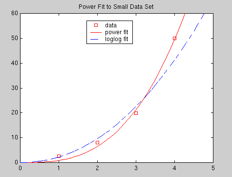
power function does, in fact, yield the minimum value of S. In the figure
below, the fits of these two power functions are compared. The fit from
Part 3 is labeled "log-log fit" and the optimal fit is labeled "power fit".

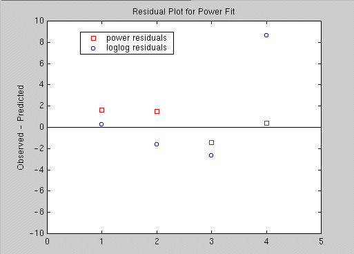
Below, we show a comparison of the residual plots of these two models.
The "log-log" model fits the data very poorly at the right end of the plot.

y = 0.921 e0.999t
|
|