|
|
|
|
|
|
Recall from the Difference Equations module that given numbers a1, a2, ... , an, with an different from 0, and a sequence {zk}, the equation
is called a linear difference equation of order n. These behave in basically the same way for doubly-infinite sequences as they do for singly-infinite sequences. As before, if {zk} is the zero sequence { ..., 0, 0, 0, ... }, then the equation is homogeneous. Otherwise, it is nonhomogeneous.
If our sequences represent sampled signals, as in Part 1, then we can think of a linear difference equation as a linear filter. The sequence {yk} is the input to the filter, and the sequence {zk} is the output of the filter.
Let

be the input
sequence. Graph both the input and the output sequences.

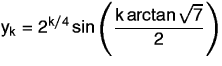
be the input
sequence. Graph both the input and the output sequences. Then
let
be the input
sequence. Graph both the input and the output sequences. What do
you observe in these two cases? Do the output sequences look like
the input sequences? Do they look like some other common
sequences? (You may need to look at your axes closely and take
round-off error into account.)
A difference equation can be regarded as a filter because, as we saw, waves with some frequencies are filtered out while others are allowed to pass unchanged. Electronic circuits that act this way are very important in many types of signal processing. For example, an equalizer on a stereo processes musical signals so that high-frequency noise is filtered out but lower frequency signals are allowed to pass.
In the next part we will show how to predict how a linear filter will behave.
|
|
|