Part 11: Solving Linear Programming Problems

Linear programming (LP) is an application of linear algebra in which the central problem is to maximize or minimize a linear function (of perhaps many variables) on a domain defined by linear inequalities and equations. In this tutorial, we consider only LP problems in two variables. In this Part, we address such problems directly in terms of linear algebra. In Part 12, we explore Maple's commands for solving such problems by the Simplex Algorithm, the central tool of applied linear programming.

Our prototypical LP problem* is this:

Problem A.  Find values of  x  and  y  that will maximize  z = 120x + 100y  subject to the restrictions

The function  z(x,y)  to be optimized is called the objective function. The inequalities that determine the domain are called constraints. Points  (x,y)  that satisfy all of the constraints are called feasible. Points that are not feasible are excluded. The variables  x  and  y  are called decision variables.

1. First we explore the geometry of the domain determined by the constraint inequalities. Maple's plots package has a command called inequal that draws such a domain. If you have already loaded the plots package in this session, you don't need to do that again. Otherwise, enter
   with(plots);
   Then enter
   constraintsA:={2*x+2*y<=8, 5*x+3*y<=15, x>=0, y>=0};
   and
   domainA:=inequal(constraintsA, x=0..5, y=0..5):%;
   The result should look something like this:

   

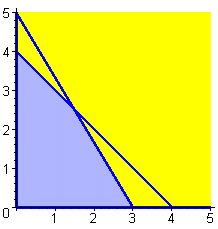
   However, the default colors are different from the ones we show here. The command that drew this picture was actually
   domainA:=inequal(constraintsA, x=0..5, y=0..5, optionsclosed=(color=blue, thickness=3), optionsexcluded=(color=yellow) ):%; 
   You may experiment with plot options to find a combination you like. ("Closed" refers to the bounding lines, and "excluded" refers to points outside the domain.) How does the picture drawn by inequal represent the feasible region?
2. Next we draw a contour map of the objective function. Enter
   contourplot(120*x+100*y,x=-1..5,y=-1..5, thickness=3, contours=6);
   and explain what the picture shows.

The "contours" or "level curves" of a linear function are just parallel straight lines. In the following figure we have superimposed the contour map on the domain plot -- which you may do in Maple by using the display command. We have also indicated the constant  z  values on the corresponding contours. [We chose contours through the points (0,0), (1,1), (2,2), etc., to make the calculations easy.]

Observe that  z  increases as we move up and to the right across the domain. The first two contours (from the left) include points in the domain, but their  z  values are clearly not maximal. The two contours on the right miss the domain entirely -- that is, they contain no feasible points. It is not clear whether the middle contour meets the domain or not, but the maximal  z  value must be close to 440. And the exact point where  z  is maximized must be the "corner" of the domain where the two slanting boundary lines meet. Thus, our job is to find that point.

Finding the point of intersection of two lines in the plane is not a difficult algebra problem. Indeed, all we have to do is solve the simultaneous equations

2x + 2y =   8

5x + 3y = 15

However, we choose deliberately to complicate the problem so that our means of solution relates to more general LP problems for which we will not be able to spot the answer by looking at a picture in the plane.

Because we are about to introduce some new variables, we rename  x  and  y  as  x₁  and  x₂,  respectively. Now we introduce  x₃  and  x₄  to represent the "slack" between the right and left sides of the inequalities. That is,  x₃  is  8 - 2x₁ - 2x₂,  and similarly for  x₄.  These new variables turn our inequalities into equations in nonnegative variables:

2x1 + 2x2 + x3          =   8

5x1 + 3x2          + x4 = 15

x1 > 0, x2 > 0, x3 > 0, x4 > 0.

Note that these equations tell us immediately the values of  x₃  and  x₄  when  x₁  and  x₂  are both  0. But what we want to know is the values of  x₁  and  x₂  when  x₃  and  x₄  are both  0.

3. Use the solve command (as in Part 9) to solve the new equations for  x₁  and  x₂.  Then read by inspection the values of  x₁  and  x₂  at the intersection of the sloping lines.
4. Find the maximal value of  z.  Did the contour  z = 440  contain any feasible points or not? Explain.
5. Apply what you have learned to solve

   Problem B.*  Find values of  x  and  y  that will minimize  z = 20x + 25y  subject to the restrictions

   2x + 3y > 18

   x + 3y > 12

   4x + 3y > 24

   x > 0, y > 0.

   Draw the domain, make a contour map of the objective function, and decide where the minimum value must be found. Introduce slack variables, and solve for  x  and  y  when the appropriate slack variables are 0.

* Problems A and B are adapted from Section 1.1 of Elementary Linear Programming with Applications, 2nd ed., by B. Kolman and R. Beck, Academic Press, 1995. The suggested context for Problem A is maximizing profit from a manufacturing product mix and for Problem B minimizing the cost of a two-food meal that meets certain nutritional constraints.

modules at math.duke.edu

Copyright CCP and the author(s), 1998-2000