Fourier, part 7

Fourier Approximations and Music

Part 7: Approximating a Periodic Function Given as a Data Set

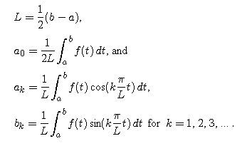
If f is a periodic function which completes exactly one period over the interval [a,b], then we can use the following formula to find the n^th approximating trigonometric polynomial

where

In many applications the function that we want to approximate is not given as a formula, but as a set of data. The following are examples.

Example 1

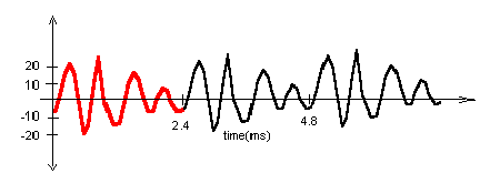
Recall that the air pressure function created by a musical instrument sounding a note can be thought of as a combination of simple sine and cosine functions, the harmonics of the sound. Suppose we want to analyze the sound of a oboe to determine its harmonic structure. We can play an oboe into a sound detector connected to a data acquisition device, e.g., a Texas Instruments CBL. This device converts the air pressure measurements into scaled voltages which are stored in a calculator or computer along with the corresponding sampling times. Below you will see the results of such an experiment. The table contains the data that corresponds to the red portion of the graph.

Oboe Graph

Oboe Data

Time (ms)	0	0.09009	0.18018	0.27027	0.36036	0.45045	0.54054	0.63063	0.72073
Sound Pressure	-7	2	16	22	17	-3	-20	-14	10

Time (ms)	0.81082	0.90091	0.99100	0.108109	1.17118	1.26127	1.35136	1.44145	1.53154
Sound Pressure	25	22	-1	-15	-13	-3	10	16	13

Time (ms)	1.62163	1.71172	1.80181	1.89190	1.98199	2.07208	2.16217	2.25226	2.34236
Sound Pressure	3	-7	-7	2	7	6	-1	-7	-6

How can we apply our integral formulas to this set of data to find an approximating trigonometric polynomial.?

Approximately what note was played on the oboe? (Recall that 1 ms = 1/1000 sec.) You may want to return to Part 2 to remind yourself how notes are named.

Example 2

Biologists have long observed that certain animal populations fluctuate periodically. An example of this is given by the Canadian lynx population during the 19^thcentury. The fur trading records of the Hudson Bay Company provide a long term account of the populations of a number of species including the Canadian lynx. We assume that the size of the lynx population in a given year is directly proportional to the number of lynx pelts purchased by the Hudson Bay outposts in that year. Below is a graph of the number of lynx pelts obtained by the Hudson Bay Company in their McKenzie River district from 1821 to 1910. The data presented correspond to the red portion of the graph.

Lynx Graph

Lynx Data

Year	1821	1822	1823	1824	1825	1826	1827	1828	1829	1830
Pelts	269	321	585	871	1475	2821	3928	5943	4950	2577

Year	1831	1832	1833	1834	1835	1836	1837	1838	1839	1840
Pelts	523	98	184	279	409	2285	2685	3409	1824	409

Year	1841	1842	1843	1844	1845	1846	1847	1848	1849	1850
Pelts	151	45	68	213	546	1003	2129	2536	957	361

Year	1851	1852	1853	1854	1855	1856	1857	1858	1859	1860
Pelts	377	225	360	731	1638	2725	2871	2119	684	299

Year	1861
Pelts	236

Estimate the period of oscillation of the lynx population.
Why would we not want to pick ten years as the period?

In each example, the information on the function is given as data. For this reason, we will need to use a numerical method to calculate the integrals for the Fourier coefficients. We will use the method known as the "Trapezoid Rule." So, before we continue with our analysis of the oboe sound and our modeling of the lynx population data, we digress for a short review of this method of numerical integration.

Graph of y = f(x)

Explain why T defined below is an approximation to the blue region under the graph y = f(x).

where delta = x₂ - x₁. In other words, why is T an approximation for the integral of f from x₁ to x₃?

In the following problem, we use the Trapezoid Rule to estimate the cross sectional area of a river. The depth of the river is measured at 5 equally spaced locations across the river. The resulting measurements along with the river's width are shown in the picture and table below.

River Profile

River Data

Distance from shore (ft)	0	13.5	27	40.5	54	67.5	81
Depth (ft)	0	10	16	19	24	18.5	0

(a) Explain why the summation in your worksheet uses the Trapezoid Rule to approximate the cross sectional area of the river.
(b) What is the relationship between the number of data points and the number of subintervals they define?
(c) Do you think the area calculated over estimates or under estimates the actual area? Explain.

We now begin our analysis of the Canadian lynx population data between the years 1821 and 1861. This population function is a good example of a periodic function whose natural domain of definition is not an interval symmetric about the origin. To find the approximating trigonometric polynomials, we will use the formulas that were established in Step 12 of Part 6 and were displayed at the beginning of this section.

(a) Enter the years and pelt numbers on your worksheet and graph the data .
(b) The lynx population appears to be periodic with period approximately 40 years. Enter the length delta of the intervals between data values, the number m of subintervals, and the half-length L of the period. (Remember that the number of subintervals is one less than the number of data points.)
(c) Explain why the formula given calculates a₀. Give an interpretation of this number in terms of lynx pelts and years.
(d) Starting with the formula for a₁,

explain how the code given on the worksheet calculates an approximate value for a₁.
(e) Modify the calculation of a₁ in order to calculate b₁.
(f) Modify the formulas for calculating a₁ and b₁ so that you can calculate general coefficients a_k and b_k for any positive integer k.
(g) Define the approximating trigonometric polynomials, and compare the graphs of these polynomials to the lynx data.
(h) Vary the order n of the approximating trigonometric polynomial. Experiment with different values of n between 5 and 30 until you are satisfied that your polynomial gives a good fit to the lynx data. Your worksheet should include at least three comparison graphs. In your conclusion explain what happened when n was too large.
(i) An important test of your approximation will be how well it can predict future lynx populations, i.e., after the year 1861. Plot the graph of your approximating trigonometric polynomial together with the lynx pelt data for the years 1821 to 1900. (Notice that the pelt data has been connected with line segments.) How well does your polynomial match the pelt data over the years 1860 to 1900? What seems to be the problem with your polynomial?
(j) If you look carefully at the data, you will see that the period of oscillation of the lynx population is less than our estimate of 40 years. Study the data, and find the number years between the two largest population surges. Use this number as the period of oscillation. Adjust the values of m and L, and recalculate a₀, a_k , b_k and your approximating polynomial. Compare this adjusted polynomial to the lynx data by replotting the graphs. Describe the results.
We now turn to the harmonic analysis of the oboe tone. Begin your analysis by finding values for delta, L, and m. Experiment with different values of n until you have one that seems to fit the data well. Show at least three comparison graphs; the one you feel best fits the data, one in which n is too small and one in which n is too large.

modules at math.duke.edu